Exploring Berkeley IGS Poll Data in Python
Between April 16 and 20, 2020 the Institute of Governmental Studies (IGS), in conjunction with the California Institute of Health Equity and Action(Cal-IHEA), polled 8,800 registered voters about a variety of issues concerning the current state of politics and COVID-19. This was an unprecendented and urgently needed pulse-taking of the California populace during the pandemic. A more recent Berkeley IGS Poll from July 2020 that follows up on these and other issues of importance to Californians was just completed.
Below we provide an overview of the Berkeley IGS Poll and describe how key findings from this survey are reported in the Berkeley IGS Poll Reports while the data itself is made available by the D-Lab.
We then provide a detailed tutorial on how to access and explore the Berkeley IGS Poll data in Python.
Introduction
About The Berkeley IGS Poll
The Berkeley IGS Poll is a periodic survey of California public opinion on important matters of politics, public policy, and public issues. The poll, which is disseminated widely to California registered voters, seeks to provide a broad measure of contemporary public opinion, and to generate data for subsequent scholarly analysis. Berkeley IGS Polls have been distributed 2-4 times per year since 2015.
The Berkeley IGS Polls continue the tradition of the California Field Polls. The Field Poll, or the California Poll, was established in 1947 by Mervin Field and operated continuously as an independent, non-partisan, media-sponsored public opinion news service from 1946 - 2014. Prior to their discontinuation, IGS collaborated with the Field Poll on a number of polls in 2011 and 2012.
Berkeley IGS Poll Reports
IGS staff and affiliates, as well as other UC Berkeley researchers, analyze the reponses from each survey and publish summary reports of key findings as part of the Berkeley IGS Poll report series. Typically many reports are produced per survey. Recent IGS Poll reports can be downloaded from eScholarship. You can stay abreast of new IGS Polls and reports by using the form on the IGS website to join the IGS mailing list.
Accessing the Berkeley IGS and California Field Poll Data
The D-Lab makes the IGS and Field Poll data available via SDA. SDA, or Survey Documentation and Analysis is an online tool for survey data analysis that also provides a platform for managing the survey data files and related documentation and facilitating their download. SDA was developed at UC, Berkeley but since 2015 it has been managed and supported by the Institute for Scientific Analysis (ISA), a private, non-profit organization, under agreement with the University of California.
A complete list of the IGS and Field polls that are accessible via SDA can be found on the D-Lab Data California Polls webpage.
Tutorial
In this section, we will show you how to download data from SDA and then import into Python for a little exploratory data analysis and map making!
Import python libraries
Before we get into the weeds, let's import the libraries we will use.
import numpy as np
import pandas as pd

import matplotlib # primary python plotting library
%matplotlib inline
import matplotlib.pyplot as plt # more plotting stuff

import requests
from urllib.request import urlopen, Request

import json # for working with JSON data
import geojson # ditto for GeoJSON data - an extension of JSON with support for geographic data
import geopandas as gpd # THE python package for working with vector geospatial data

import pyreadstat # for working with proprietary statistical software data formats
Accessing a Survey in SDA
The SDA tool can be used to access the IGS COVID-19 Poll data from April 2020 as well as any other IGS Poll data. If we check the D-Lab California Poll page, we see that the SDA URL for this poll is https://sda.berkeley.edu/sdaweb/analysis/?dataset=IGS_2020_03
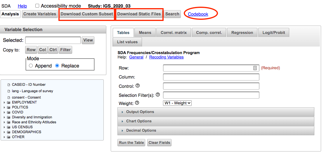
Clicking that link opens the SDA landing page for the survey which contains a number of tools for online analysis as well as a left-side panel describing the available variables. The SDA Help link provides documentation for doing online analysis.
Take a minute to notice the buttons for
downloading the dataora custom subsetand for accessing thecodebook (metadata)both of which are highlighted in the screenshot below.
Downloading Data from SDA
If you click on the Download Static Files link you will be able to download the IGS Poll data as a fixed-width text file by clicking on the Data file button. To make sense of that file you need to download a data definition file as well.
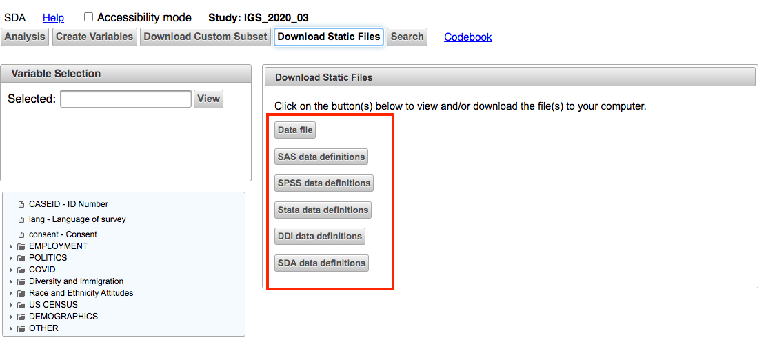
The DDI data definitions file is a XML file that uses the open-source Data Documentation Initiative specification for survey metadata. You can use the DDI file with the data file to read the data directly into Python. However, this method requires knowledge of reading in fixed width files and extracting structured data from an XML file.
Alternatively, you can download a software specific data definition file that allows you to import the data into statistical software like SPSS or Stata.
Download SDA File for SPSS
For this tutorial go ahead and download the IGS Poll data in SDA so that you can import it in SPSS and then save it as a *.SAV file.
- Download the
Data File - Download the
SPSS data definition file - Download the
codebook
Follow the instructions in this online PDF to import into the data and ddl file into SPSS and save as an SPSS sav file. You can search online for other documentation on process.
Working with the IGS Poll Data in Python
If you want to read in a proprietary statistical data file (SPSS or SAS etc) into Python you can use the pyreadstat package or similar. This process is detailed in the excellent blogpost How To Analyze Survey Data With Python, by Benedikt Droste (7/21/2019).
We will draw from and expand the work in that blog post below.
Read in SPSS file
Use pyreadstat.read_sav to read in the SPSS file created from the SDA output. As you recall SDA produced a data file and a data definition file (DDL). The contents of both of these are in the SPSS sav file igs-covid-poll-april2020_withlabels.sav. When we read this file in the function returns both a pandas dataframe (df) from the data file and a metadata object from the DDL file.
Follow along: The notebook and data for this tutorial can be found here.
# Read in the data into df and the detailed column metadata into meta
df, meta = pyreadstat.read_sav('data/igs-covid-poll-april2020_withlabels.sav')
First, take a look at the dataframe
df.head()
The meta object is a pyreadstat object that contains, among other things:
meta.column_names- A list of the column names
meta.column_labels- A list of the descriptive column labels
meta.variable_value_labels- a dict of dicts - column name keys and a mapping of response codes and values.
# Take a look at the first ten values of
# meta.column_names - A list of the column names
meta.column_names[0:10]
# Take a look at the first ten values of
# meta.column_labels - A list of the descriptive column labels
meta.column_labels[0:10]
# Take a look at an example dict from
# meta.variable_value_labels
meta.variable_value_labels['q3']
For convenience, let's read the two column lists into one meta_dict so that we can easily retrieve the column label from the column name.
Let's also create a shorter alias response_dict for the variable value labels dict of dicts.
# convert metato a dictionary of column name and label pairs
meta_dict =     dict(zip(meta.column_names, meta.column_labels))
response_dict =  meta.variable_value_labels
As an example of how we would use this, let's get the full text label for the column named Q23.
meta_dict['q23']
Wow, that's a long column label! Given this we won't replace the column names with the descriptive column labels. Instead we will just fetch them from the meta_dict when we need them.
Now let's look at the range of responses for this question.
- This will display the code and the label for the response.
response_dict['q23']
You can use a list comprehension to quickly search the meta_dict for columns (key) whose descriptive labels (val) have a specific string.
For example, let's identify columns that might relate to health care.
#Search for questions that mention masks
[(key, val) for key, val in meta_dict.items() if 'health' in val.lower()]
That's pretty handy! But you should always refer back to the
codebookyou downloaded from SDA if one was available.
Let's take a deep dive into Q23 since the results for this question were summarized in the IGS Poll Report:
Mora, G., Schickler, E., Haro, A., & Rodriguez, H. (2020). Release #2020-10: Support for a Single-Payer Health Care System to Address Disasters & Pandemics. UC Berkeley: Institute of Governmental Studies. Retrieved from https://escholarship.org/uc/item/1n25x39s
meta_dict['q23']
If we look at the value_counts for this column we get the distribution of counts across the response options.
df['q23'].value_counts(dropna=False)
We can normalize the output of value_counts to get the proportion of responses for each value.
df['q23'].value_counts(normalize=True)
Now let's use the response_dict to display human readable response values.
df['q23'].map(response_dict['q23']).value_counts(normalize=True)
Creating Tables from IGS Poll Data
We can up our game by creating a pandas crosstab to see how the responses vary by another variable. Here let's consider the political party of the survey respondent, which is in q9.
meta_dict['q9']
pd.crosstab(df['q23'], df['q9'], dropna=True, normalize='columns')
Add we can pretty up the formatting of the output..
pd.crosstab(df['q23'], df['q9'], dropna=True, normalize='columns').style.format("{:0.2f}")
Above, we normalized by column so that the column values would add up to 1 (or 100% if converted to percents).
Let's bring it home by adding pretty column labels and response labels.
pd.crosstab(
        df['q23'].map(response_dict['q23']), # The response values for q23
        df['q9'].map(response_dict['q9']),   # The response values for q9
        dropna=True, normalize='columns'). \
        style.format("{:0.2f}")              # and format the output
We can also reorder the rows so that they align with the original order of the responses.
Let's do that and save the output to a dataframe named q23_table.
q23_table = pd.crosstab(
        df['q23'].map(response_dict['q23']), # The response values for q23
        df['q9'].map(response_dict['q9']),   # The response values for q9
        dropna=True, normalize='columns').  \
        loc[response_dict['q23'].values()]. \
        loc[:,response_dict['q9'].values()]
q23_table
Now that we have saved the table as a dataframe let's do a bit more reformatting.
# Since all the row values are numeric let's convert to percents and round
q23_table = round(q23_table*100, 2)

# Move the responses to a column instead of an index
q23_table.reset_index(inplace=True)

# Remove the name of the column - set to empty string
q23_table.rename(columns={'q23':''},inplace=True)

# Rename the axis to default value of none
q23_table.rename_axis(None, inplace=True, axis=1)

# Take a look
q23_table
Let's see how that output compares to Table 1 of the IGS Report:
Mora, G., Schickler, E., Haro, A., & Rodriguez, H. (2020). Release #2020-10: Support for a Single-Payer Health Care System to Address Disasters & Pandemics. UC Berkeley: Institute of Governmental Studies. Retrieved from https://escholarship.org/uc/item/1n25x39s
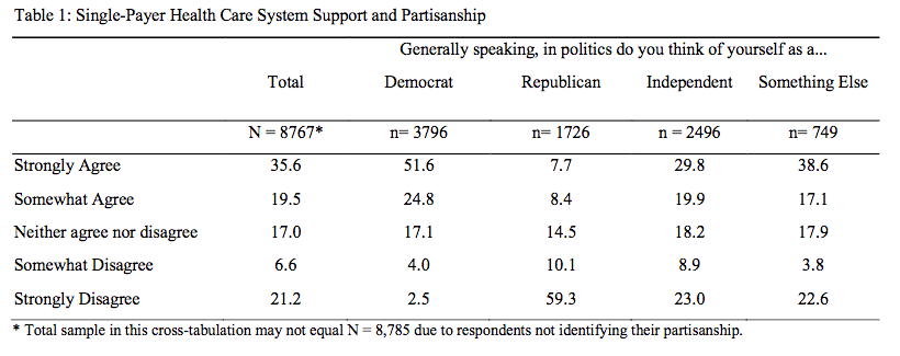
You can see that our values do not match. This is because we are not including the survey weights.
Let's weight the values, which are in the column w1, and then compare the tables again.
q23_table_weighted = pd.crosstab(
        df['q23'].map(response_dict['q23']), # The response values for q23
        df['q9'].map(response_dict['q9']),   # The response values for q9
        df['w1'], aggfunc = sum,
        dropna=True, normalize='columns').  \
        loc[response_dict['q23'].values()]. \
        loc[:,response_dict['q9'].values()]

q23_table_weighted
# Since all the row values are numeric let's convert to percents and round
q23_table_weighted = round(q23_table_weighted*100, 2)

# Move the responses to a column instead of an index
q23_table_weighted.reset_index(inplace=True)

# Remove the name of the column - set to empty string
q23_table_weighted.rename(columns={'q23':''},inplace=True)


# Rename the axis to default value of none
q23_table_weighted.rename_axis(None, inplace=True, axis=1)

# Take a look
q23_table_weighted
Now we have matching output!
Mapping IGS Poll Data
In the next section of our tutorial we will show you how to map the survey response data.
For this, we will:
- Read in the USA County cartography boundary file from the Census website.
- Subset it to include only California Counties
- Subset the survey data to keep only
q23responses byq2- which is the respondent's county. - Join the survey subset to the county data
- Map it.
We will use the Geopandas library to work with and map the geographic data.
Fetch the county boundary data and take a look.
counties = "https://www2.census.gov/geo/tiger/GENZ2019/shp/cb_2019_us_county_500k.zip"
counties = gpd.read_file(counties)
counties.plot()

Take a look at the county data so we can find a column on which to subset by state.
counties.head()
Use the California state fips code *068 to subset the county data.
counties = counties[counties['STATEFP']=='06'].reset_index(drop=True)
counties.plot()

counties.head()
Take a look at the q2 descriptive label.
meta_dict['q2']
Take a look at the set of responses for this question.
response_dict['q2']
Now we want to create the data that we wish to map using pd.crosstab.
We want the responses to Question 23 (q23) as the columns and those for Q2-county (q21) as our rows. Thus the ouput will look a little different.
IMPORTANT: Because we want the values for q23 to sum to 1 (or 100 for percentages) for each county, we now want to
normalizeby rows (or index) not by column as we did previously.
# Need to set normalize to 'index' to get correct values by county
q23_by_county = pd.crosstab(
                    df['q2'].map(response_dict['q2']),
                    df['q23'].map(response_dict['q23']),
                    df.w1, aggfunc = sum, dropna=True,
                    normalize='index')

q23_by_county =  round(q23_by_county * 100, 2) # convert to percents and round
q23_by_county.reset_index(inplace=True)

q23_by_county.head()
Next, we use the Geopandas geodataframe merge method to join the survey data to the county boundaries.
- Our join values will be the county names which are in the
q2column of the q23_by_county dataframe and in theNAMEcolumn of the counties geodataframe. - We do a "left" join to keep all the rows in the left table - here the
countiesgeodataframe.
counties_q23 = counties.merge(q23_by_county, left_on="NAME", right_on="q2", how="left")
If you take a look at the output geodataframe you can see the responses to q23 have been appended to the rows for each county.
counties_q23.head()
Now we will use matplotlib and geopandas to map of one column in the output table counties_q23: Strongly Agree, or the percent of those who strongly agree with the question.
fig, ax = plt.subplots(figsize = (8,10))
counties_q23.plot(column='Strongly Agree',
                  scheme='user_defined',
                  cmap="Reds",
                  edgecolor="grey",
                  classification_kwds={'bins':[10,20,30,40,50]},
                  legend=True,
                  legend_kwds={'title':'percent'},
                  missing_kwds= dict(color = "lightgrey"),
                  ax=ax)
ax.set_title("Percent of Californians who strongly agree that a single-payer health care system,\n such as Medicare-for-all in which all Americans would get their insurance from a single government\n plan, would improve the nations ability to respond to disasters and pandemics such as COVID-19.")
plt.show()

That map reveals some potentially interesting regional differences that could be worth investigating further. They may also be an artifact of few survey responses in those particular counties.
Making Reusable code
Finally, we can leverage our code to create functions so that we can map any question response by county.
For those of you who work with geographic data, you will see that I added a named argument
map_crsto the function with a default value for California. This allows one to set the map project of the output map to create a more custom look.
def make_county_map(gdf, column_name_str, title="no_title", map_crs='epsg:3310'):
    '''
    Create a map by county of any column in a geodataframe
    '''
    fig, ax = plt.subplots(figsize = (8,10))
    gdf.to_crs(map_crs).plot(column=column_name_str,
                  scheme='user_defined',
                  cmap="Reds",
                  edgecolor="grey",
                  classification_kwds={'bins':[10,20,30,40,50]},
                  legend=True,
                  legend_kwds={'title':'percent'},
                  missing_kwds= dict(color = "lightgrey"),
                  ax=ax)
    ax.set_title(title)

    # Remove axis clutter
    ax.set_axis_off()
plt.show()
Test our function with the geodataframe and column we just used.
make_county_map(counties_q23,'Strongly Agree', 'Respondants who strongly agree with a Single-Payer System')

Now let's create a function to create the geodataframe so we can make a map for any question-response pair.
def make_county_gdf(column_name_str):

    tempdf = pd.crosstab(
                df['q2'].map(response_dict['q2']),
                df[column_name_str].map(response_dict[column_name_str]),
                df.w1, aggfunc = sum, dropna=True,
                normalize='index')

    tempdf =  round(tempdf * 100, 2) # convert to percents and round
    tempdf.reset_index(inplace=True)
    county_gdf = counties.merge(tempdf, left_on="NAME", right_on="q2", how="left")
    return county_gdf
Let's map the percent of folks who responded that mask usage is very effective for preventing COVID-19.
# Search for questions that mention masks
[(key, val) for key, val in meta_dict.items() if 'mask' in val.lower()]
q19_1_3 looks good. Let's take a look at the response values for that question.
response_dict['q19_1_1']
Let's map that!
my_gdf = make_county_gdf('q19_1_3')
make_county_map(my_gdf,'Extremely effective', 'Respondents who believe Masks to be Effective against COVID-19')

That worked! Yeh.
Now let's flip that so we can see the geographic distribution of responses where masks are thought to be not effective.
my_gdf = make_county_gdf('q19_1_3')
make_county_map(my_gdf,'Not effective at all', 'Respondents who believe Masks are NOT effective against COVID-19')

Next Steps
There are many ways in which we could expand on this tutorial. For example, these topics come to mind:
- downloading and working with the data in CSV format so as not to require proprietary software
- creating interactive maps of the survey data
- creating publication ready plots and tables
Keep your eye on the D-Lab blog page as we plan to cover that first topic in a future post. Sign up for a D-Lab workshop this semester if you want to learn about the other topics which have more general applicabilty.
Parting thoughts
The Berkeley IGS Polls are a tremendous source of data about California public opinion and Python has great libraries for exploring these data. If you are interested in staying abreast of the Berkeley IGS Poll reports, sign up for the IGS mailing list. If you want to work with the data itself, keep your eyes on the D-Lab California Polls web page.
If you are looking to develop your data science skills, check out the D-Lab web site. Better yet, join our newsletter as well and stay abreast of our upcoming workshops as we get ready for the Fall 2020 semester.